
The Quantity Theory of Money
Examining the money supply and inflation

It’s widely accepted that the amount of money in circulation will impact the economy’s price level, but there is substantial disagreement over how strong this relationship is. If, for example, the amount of money doubles, will that double the economy’s price level? While the past several months of tightening monetary policy and a subsequent decrease in inflation may lead one to answer "yes," it’s important to consider the several additional factors that impact prices: demographic changes, geopolitics, aggregate supply, etc. This debate over the importance of the various causes of inflation leads us to one of the oldest theories in economics: the quantity theory of money.
The foundations
Dating back to the 16th-century writings of Nicolaus Copernicus (yes, the guy who came up with the sun-centric model of the universe), this deceptively simple concept emphasizes the relationship between inflation and the money supply. To be exact, it posits a direct relationship between the quantity of money in an economy and the general price level. However, the mathematical representation wasn’t formulated until the early 20th century by American economist Irving Fisher and his equation of exchange:
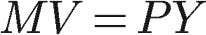
M is the amount of money, V is the velocity of money (the rate at which money is used to purchase new goods and services), P is the price level, and Y is real GDP – hence the direct relationship between the money supply and prices. There are a few things to keep in mind here before going forward. First off, PY (the price level multiplied by the real GDP) is in fact the nominal GDP. This also means that the money supply multiplied by the velocity of money yields the nominal GDP – money velocity encompasses only activities that contribute to GDP, and so multiplying that number with how much money there is (specifically, money used to purchase new goods and services) equals the nominal GDP.
Secondly, if we assume the velocity of money and the real GDP as constants, this means the relationship between M, money, and P, prices, is not only direct but also proportional. So, yes, assuming a constant velocity of money and real GDP, a doubling in the amount of money will double the economy’s price level. This may seem like a trivial point at first, but it highlights an important macroeconomic concept that countries like Zimbabwe, Hungary, and Weimar Germany failed to understand: if the government keeps producing more and more money, that doesn’t mean increased production, just higher prices.
Going back to the equation of exchange, here’s an example to make it more intuitive: let’s assume the money supply totals $100, the real GDP is $1000, and the price level is 3 (this is usually measured through an index, i.e., the Consumer Price Index).
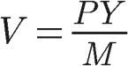

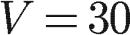
This basically means that, given the variables above, your average dollar is going to "circulate" (trade hands) 30 times per year. Because GDP is simply the value of all goods and services produced in a certain time frame, this means that those 30 exchanges had a total nominal value of $3000. To illustrate this idea further, let’s set up an even simpler situation: the money supply is $1, the GDP is $1000, and the price level is 1. The velocity of money in this case would be 1000, as the money supply of $1 would have to be used to purchase new things 1000 times to create a GDP of $1000.
An alternative approach
The equation of exchange is, as you may have guessed, a rather simplistic framework for analyzing what is an infinitely complicated correlation. And as economics has gradually grown into a statistical science over the years, researchers have refined the mathematics behind the quantity theory of money so that it can be more useful for understanding real-world economic phenomena. One such revision is like so:

Let’s break this down.
Money supply (M): the total quantity of money in the economy
Velocity of money (V_T): the rate at which money is used to purchase new goods and services within a given time period, T
Summation operator (∑): adds up the product of the price level (p_i) and the quantity of goods and services produced (q_i) for each time period “i” from 1 to n. The product of these values yields the nominal GDP, and with the sum operator, we can get the nominal GDP across different time periods (hence the “i”)
Transpose operator (T): converts row vectors into column vectors and vice versa like so:

In this context, we’re dealing with 2 vectors: p (representing the price levels for each time period) and q (representing the quantities of goods and services produced for each time period). As previously stated, for any given time period, we need to take the product of the price level and the quantities of goods and services; to perform this operation across entire vectors, we must take their dot product. To be clear, because we’re dealing with simple row vectors, the transpose operator isn’t a necessary step; it simply adds assurance that the data works in both row and column format. Consider the following example:
Price level vector (p):
Quantity vector (q):

If we were to use the transpose operator, here’s what would happen:
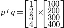
This gives us (1 x 100) + (2 x 200) + (3 x 300) + (4 x 400) = $3,000; the nominal GDP of this hypothetical economy is $3,000. Using vectors in the quantity theory of money is hugely beneficial for statisticians looking to incorporate real-life data points across several time periods when analyzing the relationship between the money supply and price levels. The equation essentially states that the total spending on goods and services (money supply multiplied by the velocity of money) is equal to the total monetary value of economic output (the sum operator). This reflects the core concept of the quantity theory of money, which literally states in the original equation that the total spending on new goods and services (MV) equals the monetary value of economic output (PY).
Keynes and company
Remember how we mentioned a "substantial disagreement" between economists as to how strong the relationship was between the money supply and prices? The quantity theorists figure it’s a pretty strong correlation, so here goes the flip side of that argument. John Maynard Keynes, arguably the most influential economist of all time, wasn’t a fan of the quantity theory of money (so it’s no wonder that Milton Friedman, who criticized several Keynesian theories, was the chief proponent of the quantity theory of money in the 1960s).
In his "The General Theory of Employment, Interest, and Money," Keynes observed how the quantity theory of money assumes people hold onto money solely to engage in transactions (hence the velocity of money in the equation of exchange) and argued that this wasn’t accurate. Rather, people may also hold onto money simply to have liquid cash on hand, particularly when things are uncertain. People want money not just as a medium of exchange but also as a store of value.
He also felt that the role interest rates play in determining the demand for money shouldn’t be overlooked. This is called the liquidity preference theory; people prefer to hold their wealth in liquid cash, but the opportunity cost of doing so is the income they would have earned in interest had they put that money in interest-bearing assets like bonds or a savings account. Thus, as interest rates rise, the opportunity cost of holding money increases, encouraging people to invest in interest-bearing assets. When interest rates drop, the demand for money increases as the forgone interest income is lowered. This all means that changes in the money supply may not have a straightforward effect on prices, as interest rates can play a central role in the demand for money.
This focus on the demand for money was shared among Keynes and economists Alfred Marshall (Keynes’s intellectual forefather) and Arthur Cecile Pigou (Keynes’s professor), all of whom were from Cambridge University (which is commonly associated with Keynesian economics).
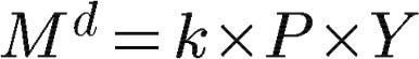
This is called the Cambridge cash-balance theory. The demand for money, M^d, is equal to the proportion of nominal income (income not adjusted for inflation) that people want to hold as cash (k) multiplied by the price level (P) multiplied by the real national income (Y). In other words, people’s demand for money is influenced by the price level (people tend to hold more money during inflation to cover increasing costs), their real income (the demand for money increases as real incomes rise because people would want to hold more money to support the increased spending at higher incomes), and the fraction of income that people prefer to hold as money.
If we assume monetary equilibrium (that is, the demand for money is equal to the money supply), the real national income is exogenous (a variable that’s determined outside the model but nonetheless imposed on the model). In this case, if Y is not influenced by other variables in the equation and k is relatively constant, then the Cambridge cash-balance theory equals the equation of exchange with one small change: the velocity of money is the inverse of the k value.
Because the demand and supply of money are equal, we can sub in the M from the equation of exchange with "k x P x Y" from the Cambridge equation:
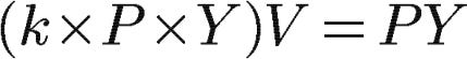
To solve for V, it’s simple algebra:

This relationship between the 2 equations demonstrates how the velocity of money is influenced by people’s preferences for holding money, as represented by k.
Econ IRL
A key facet of a country’s immigration policy is preparing the labor market for an influx of job seekers. The task is to figure out how to provide employment to immigrants so that they can not only gradually assimilate into the country but also best utilize their talents and skills. But what factors go into such an undertaking? This week’s paper may have an answer.
The authors studied the migration of Jews from the Soviet Union to Israel during the 1990s after the former’s dissolution and then touched base with them in 2019 to see where they ended up. There are initially clear differences between immigrants and natives in terms of labor market performance; immigrants tended to land jobs in lower-paying firms (differential sorting) and also received lower premiums than natives within firms (differential pay-setting). Moreover, by isolating for discrepancies in non-wage amenities received by immigrants and natives, the authors also deduce a desirability gap among firms: even when keeping pay constant, immigrants initially find employment at firms providing lower utility through perks.
But these gaps didn’t last long. Because immigrants change jobs more often than natives and are also more conditional on job switches (i.e., demanding higher positions), many immigrants were able to close the wage gap within a single generation. The authors do note, however, that these variables may have only been able to work their magic in this specific case study; comparing immigrants’ job mobility to natives’ is typically challenging because of migration regulations complicating things, but not here. Former Soviet Union immigrants became Israeli citizens on arrival, providing "unconstrained assimilation" undistorted by migration laws. But because immigrant-specific rules often inhibit their job mobility, it’s possible that these labor market patterns won’t replicate themselves in other countries.
‘Till next time,
SoBasically
pluh