


The intricacy of options pricing is nothing new to this blog. We briefly touched on it in our article on derivatives and further explored the topic in relation to arbitrage for our hedge fund piece. But today we’re going all in. The science of option valuation is part of the broader field of mathematical finance, utilizing methods such as stochastic calculus and Fourier analysis to calculate the intrinsic value of an option. Introducing one of the most important equations in all of finance, the Black-Scholes model.
The origin story
Originally developed in 1973 by economists Fischer Black and Myron Scholes, the idea of the Black-Scholes model was originally published “The Pricing of Options and Corporate Liabilities”, but most of the underlying math and the applications of the model was fleshed out in “Theory of Rational Option Pricing” by Robert C. Merton.
Following the model’s publication was a boom in options trading and, much later, the Nobel Prize being awarded to Merton and Scholes (Black had unfortunately passed away). But what makes the Black-Scholes model worthy of such a prestigious accolade? Although people were trading options long beforehand, there was never a clear framework as to how they should be valued.
That’s what Black-Scholes did; it showed that there exists a “fair price” for any given option and, in doing so, set the bedrock for modern option markets.
The technicals
Before getting to the actual equation, it’s important to first understand how the model conceptually works. Its underlying principle is continuously revised delta hedging, that is, offsetting the risk of holding an option by buying and selling the underlying asset in very specific ways. The portfolio’s delta (how sensitive the option price is to changes in the underlying asset’s price) should be minimized and, ideally, have an opposite sign to that of the option’s delta.
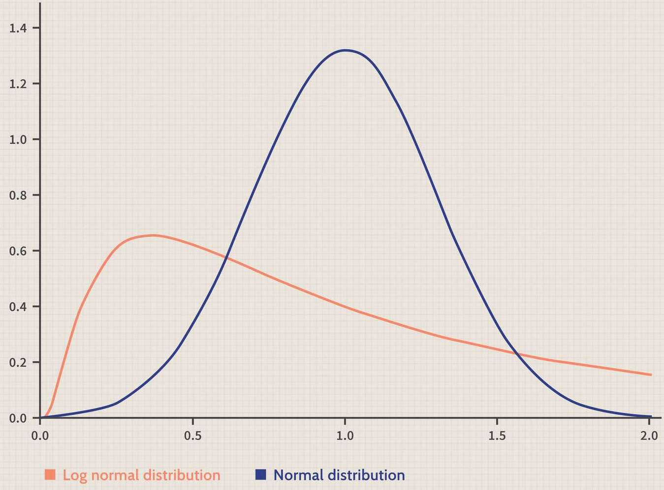
In calculating the option’s price, Black-Scholes assumes that financial instruments have a lognormal distribution of prices; a set of probabilities where their logarithms are normally distributed (a probability distribution where the values have a symmetric shape around the mean). Why make that assumption? A couple of reasons. Firstly, a lognormal distribution of option prices implies a normal distribution of option returns. Under a lognormal distribution, if a random variable x (i.e. an option’s price) is lognormally distributed, then y = ln(x) (i.e. an option’s return) is normally distributed. We’re deliberately hand waving a lot of the math here for the sake of simplicity, so don’t worry if you’re not understanding why
Secondly, lognormal distributions are bound by zero, making them convenient for modelling asset prices, which also cannot have negative values. As seen below, this is also why lognormal distributions are skewed to the right:
All you really need to keep in mind is Black-Scholes assumes option prices to have a lognormal distribution and they are bounded by zero. There are additional assumptions worth mentioning:
No dividends are paid during the option’s lifetime
No transaction costs in purchasing the option
Market price movements are fundamentally random (more on this later)
The risk-free interest rate (theoretical rate of return with zero risk. In the US, this is often denoted with the US Treasury bill rate) is constant
The option is European and can thus only be exercised when it expires (which is far easier to represent in mathematical terms than American options, which can be exercised at any point)
Now for the actual equation, it consists of 5 variables: volatility, the price of the underlying asset, the option’s strike price (the fixed price at which an option owner can buy or sell the underlying asset), the time until the option expires, and the risk-free interest rate. When it’s put all together, here’s what we get:

We get the call option’s price (“C”) by multiplying the stock price (“S”) with the cumulative distribution of d1 (we’ll get to this), and subtract it by the strike price (discounted to the current time through “-rt”: the risk-free return multiplied with the time until maturity) multiplied with the normal distribution of d2.
It’s remarkably intuitive when thinking about the intrinsic value of a call option – the underlying stock price minus the option’s strike price. The higher the stock price, the greater the likelihood that we’re going to exercise the call option and thus, the more valuable that contract is.
Say I have a call option with a $50 strike price (meaning I have the right, but not the obligation, to purchase the shares at $50) and the stock price goes to $150. The option’s value is going to increase as the owner can now buy the shares at a discount. It follows that the greater the difference between the stock price and the strike price, the more valuable the option is.
The equation has 2 parts to it: the current stock price and the option strike price, both of which have probabilities d1 and d2 attached to them:


All the variables are the same, with “ln” representing the natural logarithm of the ratio from the stock price s to the strike price k.
The sigma symbol represents the stock’s price volatility, which we find through the stock price’s standard deviation (a measurement of the variation in a set of values). Usually investors calculate this by analyzing a company’s previous stock price data, but the Black-Scholes model takes a different approach. Instead of analyzing past standard deviation in the stock prices, we analyze the future standard deviation in the stock prices, or rather, the expected future standard deviation.
As crazy as it sounds, this isn’t an attempt at predicting the future. While we don’t know the volatility, we do know the current market price for the option as options are traded non-stop. If we have that price (“C”), we can simply solve for the sigma value. That value is the implied volatility – how likely the market thinks the price of the underlying asset is going to change. And we know this value is at least somewhat accurate because it’s reflected in the market price of a given option.
So rather than solving the Black-Scholes model to get the option’s price, we reverse the Black-Scholes model to find the implied volatility by substituting the market option price. This can be very helpful in comparing various options prices as well as getting an idea of how the market feels about the underlying asset (specifically, how likely it’s going to move).
So let’s take a step back: we know that sigma denotes the underlying asset’s implied volatility. If sigma increases, then the overall probabilities d1 and d2 will increase and decrease, respectively. When d1 is plugged into the cumulative distribution function, we get the expected value of buying the stock at maturity, if and only if the option finishes in the money (possessing intrinsic value and presenting a profit opportunity). When d2 is plugged into the function, we get the probability of the stock price being at or above strike price at maturity, and therefore the probability of the call option being exercised (why would you exercise a call option if the stock price is below the strike price?).
To maximize the call option price, the d2 probability needs to be minimized because European call options can only be exercised when they expire. Think of it like this: If you can make more money selling your call option than simply waiting for it to expire, you would sell your call option. We can infer that C is of high value. But if you wait to exercise your option, that suggests a lower call option value.
As the stock value S and volatility increases, the value C of the option increases. The larger the term SN(d1), the larger the value of C. Conversely, the smaller the term K^(-rt)N(d2), the greater the value of C. So, maximizing d1 and minimizing d2 will maximize C, since the respective term of d2 is being subtracted from that of d1.
When the stock price S increases, ln(s/k) (part of both the d1 and d2 equations) increases, making d1 larger. As volatility increases, the numerator of d1 also increases, whereas the numerator of d2 is decreased because it subtracts the volatility. As a result, when stock price S and volatility increases, d1 is greater and d2 is smaller, so c, the difference of two terms involving d1 and d2, is greater.
And that’s really the essence of the Black-Scholes model: mathematically modelling the phenomenon of a higher stock market price minus the strike price giving a higher call option price. It goes without saying, of course, that in terms of the nitty-gritty mathematics underpinning the Black-Scholes model, we’ve hardly scratched the surface.
But we didn’t want this article to turn into a dissertation, so we tried to avoid as much of the math as possible. Do note that our overview of the Black-Scholes model is intended to provide a more intuitive feel as to what this formula does, rather than serve as a guidebook for how to wield these tools in the real world.
Econ IRL
Cash transfers – direct transfer payments to eligible citizens – are a popular welfare policy as it provides people the freedom to spend the money however they so choose. The impact of cash transfers on the labor market, however, are often a major point of contention between those who support and oppose these kinds of programs.
This week’s paper gets right in the middle of this question. The Czech Republic recently increased the cash transfers for parents by 36% without any conditions on the recipient's employment status. The authors study the effects of the newly-introduced benefits and find that the labor market participation of mothers of young children decreased by 15%, while hours worked fell by 16%.
‘Till next time,
SoBasically