


The situations and hypotheticals used in our game theory series thus far have been rather unrealistic. Just for those of you who don’t know, it’s quite rare for a striker’s teammates to be significantly less impressed because he scored left and not right. This week’s game theory model, on the other hand, actually originated from a real-life scenario.
Cournot competition has the following features:
More than one firm, each producing homogenous products (meaning there’s no product differentiation between the firms)
No collusion
Firms have market power and are able to affect the good’s price depending on their output decisions
A fixed number of firms
Firms compete more so in the quantities they produce rather than the prices of goods
Before mathematically setting this model up, we must recognize what Cournot competition actually is: a market structure where firms independently decide and compete on the amount of a product or service they will produce.

Think of this as the profit-maximizing function. With P being price, Q being the total quantity firms produce, C being marginal cost, and i being the firm, this expression is saying price multiplied by the firm’s quantity minus that firm’s marginal cost. From here we can set this up into a game of sorts. Say we have couple of players, Firm #1 and Firm #2, that both operate in accordance with the profit-maximizing function. In order to maximize profit, Firm #1 is deriving the best response to Firm #2’s output decision.
Let’s break down the profit-maximizing function:

P or price comes from a - Q. Hence, the price function is P(Q) = a - Q, where a is a constant, representing what the consumer is willing to pay. Once we subtract out Q, we have our price. Now because we’re subtracting Q from the price the consumer is willing to pay, we can intuitively conclude that as the quantity increases, the price decreases. Think about it in terms of simple supply and demand: you have more of something, it becomes less rare and so people tend to value it less.
But within this expression, we get Q by adding Q1to Q2 (the production quantities of Firm #1 and Firm #2, respectively). Why? Remember, we’re dealing with homogenous goods, so consumers don’t care which brand they’re coming from, they’re only interested in the price. As such, it’s the total quantity of the good out there that determines the good’s price:

From here we want to rearrange the expression such that it becomes easier for us to focus on what is actually being sought after, like so:

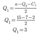
What we’re trying to figure out is the value of Q1 - what production point is most optimal for Firm #1? With the expression above, we can visually answer that question. Let’s set a to $15, Q2 to 7, and C1to $2. In other words, the consumer is willing to pay no more than $15, Firm #2 is producing 7 units of the good, and we have a marginal cost of $2. If we just plug in these numbers, we get a quadratic function:


If we graph it, replacing the Qs with Xs in the process:

What is this graph telling us? Firm #1’s optimal production point is 3 units of the good at $9 each. We can even work this out mathematically without using graphs and instead employ derivatives. Without getting too lost into the weeds here, the derivative of something is where a variable's power becomes its coefficient. So the derivative of X^2 would be 2X, for example. Let’s apply this to our broken down profit-maximizing function:

The reason we’re not including the derivatives for Q2, C1 or a is because those variables are constant. From we here just solve for Q1, plug in our variables, and we should get 3:
Let’s quickly do the same for Firm #2 (assuming that their marginal cost is say, $4):
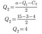
Thus, Firm #2’s optimal production point, given what Firm #1 is produced at, is 4 quantities. Now that we have both firm’s optimal responses, we can derive an equilibrium. Recall what that term means in the context of game theory: when firms are in equilibrium, neither of them want to change what they’re doing given the other firm’s strategy. What we essentially have are 2 different equations, each with an unknown variable, that need to be combined somehow.

Doing the same for Q2 by reversing the variables like so:
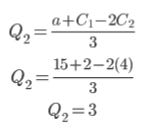
These are the optimal production points for both firms given what the other firm is going to produce. So we can now go tell Firm #1 that they ought to produce 5 units of the good because Firm #2 is going to produce 3 units of that good and vice versa, hence returning the Cournot model equilibrium.
Econ IRL
In January 2018, US President Donald Trump implemented tariffs on China to compel the CCP to stop its allegedly unfair trading practices and intellectual property theft, as well as to lower the US’s trade deficit and to advance America’s position in the technology sector. These policies were rather controversial even within the Republican Party as it marked a sharp divide between the populists and establishment members. But the name of this trade war, the US-China trade war, is rather misleading. If we were to take it at face value, it would appear as if the US and China are the only real stakeholders in the situation. This week’s paper, put together by 5 economists, show how that isn’t at all the case.
Using product-level data to analyze big-picture shifts in trade and firm-level data to study microeconomic forces such as firm investment, the authors make a particularly interesting discovery. As expected, the US and China reduced their exports to each other, but this meant that they reallocated them to other parts of the world. Although such an observation may seem obvious and insignificant, it in fact disproves the concern that the US-China trade war would end the era of global trade. If anything, the researchers argue, new opportunities for trade were created as both the US and China were incentivized to seek partners asides from each other.
‘Till next time,
SoBasically